Causal inference in panel data with heterogeneous treatment effects
Author
Vincent Arel-Bundock
Published
February 15, 2021
This notebook shows how to use R to apply and visualize two related strategies for causal inference in time-series cross-sectional data:
The “Counterfactual Estimators” described in Liu, Wang, and Xu (2020)
The “Group-Time Average Treatment Effect” estimators for staggered Difference-in-Differences introduced by Callaway and Sant’Anna (2020)
Both of these approaches are attractive because they allow us to explore treatment effect heterogeneity.
Warning: This post does not compare the performance of alternative estimation strategies, it only illustrates their application. For this purpose, I consider a single dataset simulated to match an interactive fixed effects structure; this data generating process may not satisfy the assumptions of all the methods shown below (e.g., parallel trends).
Background: Two-way fixed effects
A common strategy to analyze time-series cross-sectional data is estimate a two-way fixed effects model:
where \(Y\) is the outcome, \(D\) a binary treatment, \(X\) a vector of time-varying covariates, \(\alpha\) unit fixed effects, \(\xi\) time fixed effects, and \(\varepsilon\) noise.
Many researchers treat the two-way fixed effects model as a sort of “generalized” difference-in-differences estimator, and they interpret \(\hat{\delta}\) as an estimate of the Average Treatment effect on the Treated (ATT). This interpretation only holds if several conditions are satisfied, including linearity, absence of time-varying confounders, parallel trends, and constant treatment effects.
The constant treatment effects assumption, in particular, has received much attention in recent years. Several authors have shown that when effects vary across individuals, groups, or time periods, the estimate obtained via two-way fixed effects can be biased (Chernozhukov et al. 2013; Strezhnev 2018; de Chaisemartin and D’Haultfœuille 2020). Indeed, when treatment effects are heterogeneous, the estimate \(\hat{\delta}\) can be seen as a weighted ATT, which depends on treatment group/cohort sizes, and on treatment variance and timing across treatment cohorts (Goodman-Bacon 2018).
Liu, Wang, and Xu (2020) and Callaway and Sant’Anna (2020) propose alternative estimation strategies that allow us to explore treatment effect heterogeneity.
Simulated data
Throughout this notebook we will consider simulated data which match the design in Liu, Wang, and Xu (2020) . The key features of the data are:
250 units and 35 times periods, with binary treatment \(D_{it}\), outcome \(Y_{it}\), and covariates \(X_{1it}\), \(X_{2it}\).
Half of units are never treated, and the rest are assigned to 6 cohorts who receive treatment at different times. Treatment is irreversible and there is no treatment spillover across time or units.
The treatment effect \(\delta_{it}\) varies at the individual level and tends to increase linearly in post-treatment years.
The full simulation code is copied at the bottom of this notebook. Here are the first 5 rows of one simulated dataset:
library('data.table')set.seed(1000)dat =simulate()dat[1:5, .(unit, time, Y, D, X1, X2, δ)]
In the above data, the δ column is the true causal effect for each observation.
As a reference point, we compute a simple two-way fixed effects model using the fixest::feols function,
library('fixest')mod =feols(Y ~ D + X1 + X2 | unit + time, dat)coef(mod)
       D       X1       X2
1.889978 1.007072 2.971086
Let’s save this result and the capital-T “Truth” in a data.table so we can plot them later:
att = dat[, .(Truth =mean(δ)), by =`Time after treatment`]att[`Time after treatment`>=0, `2-way FE`:=coef(mod)["D"]][`Time after treatment`<0, Truth :=0]
Counter factual estimators
Liu, Wang, and Xu (2020) describe a class of existing estimators for the ATT, and present those estimators in a unified conceptual framework. The key idea is to impute counterfactual outcomes under no treatment for units which have actually received the treatment, and to use those counterfactual outcomes to estimate individual-level treatment effects which can then be aggregated.
This general strategy works in 4 steps:
Use the untreated observations to fit a model of the outcome \(Y_{it}\).
Use this model to predict the counterfactual potential outcomes \(\hat{Y}_{it}(0)\) for treated observations.
Estimate the individual treatment effects in the subset of actually treated observations: \(\hat{\delta}_{it}=Y_{it}-\hat{Y}_{it}(0)\).
Average the individual estimates to obtain an ATT of interest.
In Step 1, analysts can use the model of their choice, and each model will carry its own identifying assumptions. In their article, Liu, Wang, and Xu (2020) consider three possibilities: (1) Two-way fixed effects, (2) Interactive fixed effects, and (3) Matrix completion.
Step 4 allows considerable flexibility in interpretation: We can average individual estimates in a given year to estimate the year-specific ATT, or within cohorts to obtain a cohort-specific estimate. This will allow us to draw nice plots.
We will now see how to compute counter factual estimates using all three of the approaches proposed by Liu, Wang, and Xu (2020).
The first estimator that Liu, Wang, and Xu (2020) consider is extremely easy to compute. We follow the 4 steps laid out in the previous section.
Step 1: Use the untreated observations to fit a model of the outcome \(Y_{it}\).
mod =feols(Y ~ X1 + X2 | unit + time, dat[D ==0])
Step 2: Use this model to predict the counterfactual potential outcomes \(\hat{Y}_{it}(0)\) for treated observations.
dat[, Y0hat :=predict(mod, newdata = dat)]
Step 3: Estimate the individual treatment effects in the subset of actually treated observations: \(\hat{\delta}_{it}=Y_{it}-\hat{Y}_{it}(0)\)
dat[, treatment_effect := Y - Y0hat]
Note that the code block above calculates the gap between \(Y_it\) and the counterfactual \(\hat{Y}_{ij}(0)\) for every unit, including the untreated one. In principle, the estimator should produce estimates of 0 in the pre-treatment period. This idea allows us to conduct diagnostic tests.
Step 4: Average the individual estimates to obtain an ATT. Here, we calculate a specific ATT for each time period relative to the first period when a unit is treated:
tmp = dat[, .(`LWX: Fixed Effects`=mean(treatment_effect)), by =`Time after treatment`]att =merge(att, tmp, all =TRUE)
Under conditions similar to those required by the standard 2-way fixed effects model, but allowing for treatment effect heterogeneity, this FEct estimate is unbiased and consistent (Liu, Wang, and Xu 2020).
Interactive fixed-effect counterfactual estimator
The second counterfactual estimator that Liu, Wang, and Xu (2020) consider is a factor-augmented model that aims to relax the no-time-varying-confounder assumption. Steps 2, 3, and 4 are the same as in the previous section, but we use a model of this form in Step 1:
where \(f_t\) and \(\lambda_t\) are factors and factor loadings. The authors highlight the conditions necessary for consistency, sketch out an algorithm to compute this model, and published an R package called fect that can be used to compute the interactive fixed-effect counterfactual estimator (IFEct):
library('fect')mod_ife =fect( Y ~ D + X1 + X2, data = dat, index =c("unit", "time"),method ="ife")# save results for plotting latertmp =data.table(`Time after treatment`= mod_ife$time,`LWX: Interacted Fixed Effects`= mod_ife$att)att = tmp[att, on = .(`Time after treatment`)]
Matrix completion counterfactual estimator
The third counterfactual estimator relies on the Matrix Completion approach of Athey et al. (2017). Once again, the fect package allows us to swap in a new model in Step 1:
mod_mc =fect( Y ~ D + X1 + X2, data = dat, index =c("unit", "time"),method ="mc")# save results for plotting latertmp =data.table(`Time after treatment`= mod_mc$time,`LWX: Matrix completion`= mod_mc$att)att = tmp[att, on = .(`Time after treatment`)]
Group-Time Average Treatment Effect
Callaway and Sant’Anna (2020) recently published an article in the Journal of Econometrics, and their approach seems in the same spirit as that of Liu, Wang, and Xu (2020). In their article, C&S define a causal quantity of interest called the “group-time average treatment effect” (\(ATT(g,t)\)). For members of particular group \(g\) at a particular time \(t\), this parameter is:
\[
ATT(g,t)=\mathbb{E}[Y_t(g) - Y_t(0)|G_g=1]
\]
One benefit of this disaggregated definition is that it allows us to build higher-level estimates by, for example, aggregating across groups or at the time period level.
To estimate the group-time average treatment effect, Callaway and Sant’Anna (2020) impose a few assumptions: (1) irreversibility of treatment, (2) random sampling, (3) limited treatment anticipation, (4) overlap, and (5) conditional parallel trends based on a “never-treated” or a “not-yet-treated” group.
If these assumptions hold, the authors show that the \(ATT(g,t)\) can be recovered by carefully selecting the groups that are leveraged for comparison. The authors propose three alternative approaches to doing this: outcome regression, inverse probability weighting, or doubly-robust. In a first step, the analyst estimates an outcome (and/or treatment assignment) model. Then, they plug-in the fitted estimates from that model into the sample analogue of the \(ATT(g,t)\) of interest.
As Callaway and Sant’Anna (2020) point out, one of the main benefits of the Group-Time Average Treatment Effect is that it can be aggregated to provide meaningful inference at different levels. For instance, in the previous section we calculated ATTs at the time-period level. We can do the same here with the aggte function:
es <-aggte(mod, type ="dynamic")# save results for plotting latertmp =data.table(`Time after treatment`= es$egt, `Callaway & Sant'Anna`= es$att.egt)att = tmp[att, on = .(`Time after treatment`)]
Visual representation of results
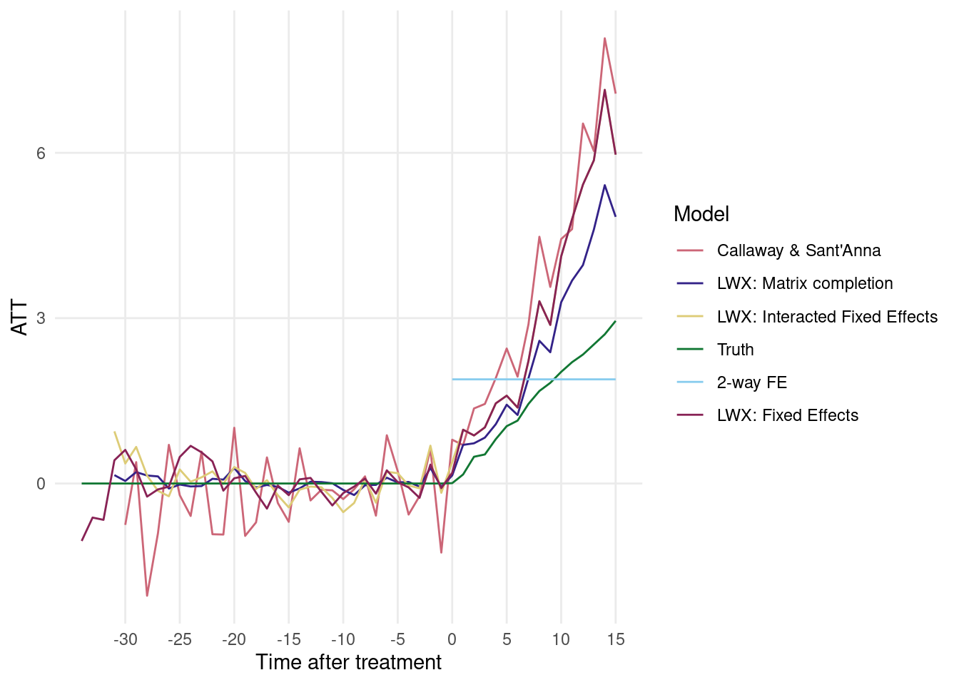
Analysts who study panel data often draw “dynamic treatment effects” plots. These plots typically show the regression coefficients obtained by interacting a treatment group membership dummy with a series of dummy variables indicating time periods relative to the period when each unit was first treated. To draw these plots, analysts must make parametric assumptions and somewhat arbitrary choices about omitted categories and binning.
The strategies advocated by Liu, Wang, and Xu (2020) and Callaway and Sant’Anna (2020) allow us to circumvent these decisions by simply plotting the estimated time-specific ATTs. I conclude by showing what this plot can look like:
library('ggplot2')tmp =melt(att, id.vars ="Time after treatment", variable.name ="Model", value.name ="ATT")palette =c("#CC6677", "#332288", "#DDCC77", "#117733", "#88CCEE", "#882255", "#44AA99")ggplot(tmp, aes(`Time after treatment`, ATT, color = Model)) +geom_line() +scale_x_continuous(breaks =seq(-30, 15, by =5)) +scale_color_manual(values = palette) +theme_minimal() +theme(panel.grid.minor =element_blank())
Simulated data
simulate =function() {# dimensions N =250 T =35# factor loadings λ_1i =rnorm(N) λ_2i =rnorm(N)# factors with stochastic drift a_t =rnorm(T)for (k in2:length(a_t)) { a_t[k] = a_t[k -1] + a_t[k] } f_1t = a_t +0.1*1:T +3 f_2t =rnorm(T)# time fixed effects with stochastic drift a_t =rnorm(T)for (k in2:length(a_t)) { a_t[k] = a_t[k -1] + a_t[k] } ξ_t = a_t +0.1*1:T +3# pre-treatment periods α_i =rnorm(N) ω_i =rnorm(N) tr_i = λ_1i + λ_2i + α_i + ω_i tr_i =rank(tr_i) /length(tr_i) T_0i =fcase(tr_i <= .5, 35, .5< tr_i & tr_i <= .6, 32, .6< tr_i & tr_i <= .7, 29, .7< tr_i & tr_i <= .8, 26, .8< tr_i & tr_i <= .9, 23, .9< tr_i, 20)# unit-specific data unit =data.table(unit =1:N, T_0i, α_i, ω_i, λ_1i, λ_2i)# time-specific data time =data.table(time =1:T, ξ_t, f_1t, f_2t)# panel data dat = unit[CJ(unit, time =1:T), on = .(unit)] dat = time[dat, on = .(time)] dat[, ε :=rnorm(N * T)][ , X1 :=rnorm(N * T)][ , X2 :=rnorm(N * T)][ , D :=fifelse(T_0i < time, 1, 0)][ , δ :=0.2* (time - T_0i) +rnorm(N * T)][ , Y :=5+ δ * D +1* X1 +3* X2 + λ_1i * f_1t + λ_2i * f_2t + α_i + ξ_t + ε] dat[, `Time after treatment`:= time - T_0i]return(dat)}
References
Athey, Susan, Mohsen Bayati, Nikolay Doudchenko, Guido Imbens, and Khashayar Khosravi. 2017. “Matrix Completion Methods for Causal Panel Data Models.”arXiv:1710.10251 [Econ, Math, Stat], October. http://arxiv.org/abs/1710.10251.
Callaway, Brantly, and Pedro H. C. Sant’Anna. 2020. “Difference-in-Differences with Multiple Time Periods.”Journal of Econometrics, December. https://doi.org/10.1016/j.jeconom.2020.12.001.
Chernozhukov, Victor, Iván Fernández‐Val, Jinyong Hahn, and Whitney Newey. 2013. “Average and Quantile Effects in Nonseparable Panel Models.”Econometrica 81 (2): 535–80. https://doi.org/https://doi.org/10.3982/ECTA8405.
de Chaisemartin, Clément, and Xavier D’Haultfœuille. 2020. “Two-Way Fixed Effects Estimators with Heterogeneous Treatment Effects.”American Economic Review 110 (9): 2964–96. https://doi.org/10.1257/aer.20181169.
Goodman-Bacon, Andrew. 2018. Difference-in-Differences with Variation in Treatment Timing. 25018. National Bureau of Economic Research. https://doi.org/10.3386/w25018.
Liu, Licheng, Ye Wang, and Yiqing Xu. 2020. “A Practical Guide to Counterfactual Estimators for Causal Inference with Time-Series Cross-Sectional Data.”SSRN Electronic Journal. https://doi.org/10.2139/ssrn.3555463.
Strezhnev, Anton. 2018. “Semiparametric Weighting Estimators for Multi-Period Differencein-Differences Designs.” In Annual Conference of the American Political Science Association, August. Vol. 30.