Regression adjustment in experiments

The other day, Jonathan Roth asked why the interacted regression adjustement strategy advocated by Lin (2013) was not more popular in experimental settings. In that thread, Lihua Lei pointed readers to an interesting new paper on the topic by Negi and Wooldridge (2020). The present notebook has three objectives:

1. Briefly summarize the headline claims from Freedman (2008b), Freedman (2008a), Lin (2013), Negi and Wooldridge (2020)
2. Show how to estimate the interacted regression adjustement model advocated by Lin and N&W using R.
3. Replicate a Monte Carlo simulation from N&W to illustrate the finite sample properties of the estimator in question.

Three estimators

In the simulations below, we will consider a case with an outcome \(Y\) and two covariates \(X_1,X_2\). The treatment \(W\) is a Bernoulli random variable, so it is independent of the covariates and potential outcomes: \(W\perp\{X_1,X_2,Y(0),Y(1)\}\). We want to estimate the Average Treatment Effect of \(W\) on \(Y\) using linear regression. The questions are:

Should our linear regression model adjust for \(X_1\) and \(X_2\)? If so, how?

The primary goal of regression adjustment in experimental settings is to improve the precision of our estimate of the treatment effect. However, in a pair of widely read papers, David Freedman argued that regression adjustment can be unwise (Freedman 2008b, 2008a). His abstracts are rather brutal:

“Regression adjustments are often made in experimental data. Since randomization does not justify the models, bias is likely; nor are the usual variance estimates to be trusted” […] “Adjustment may improve precision, or make precision worse; standard errors computed according to usual procedures may overstate the precision, or understate, by quite large factors.”

Negi and Wooldridge (2020) summarize the two main issues raised by Freedman as follows:

1. With randomization, the simple difference in means estimator is unbiased, as long as there are some units in both the control and treatment groups. In contrast, regression adjusted estimators are only guaranteed to be consistent, and they can be biased in small samples unless the conditional expectation function is correctly specified and linear in parameters.
2. The regression adjusted estimator may not always improve over the simple difference in means in terms of asymptotic efficiency.

In practice, these problems are likely to be worse when the number of subjects in the treatment and control groups differ, when treatment effects are heterogenous at different levels of the covariates, and if the linear model is misspecified.

Lin (2013) acknowledges the possibility of small sample bias (problem #1), but argues that the problem “diminishes rapidly with the number of randomly assigned units” (order 1/n). According to Lin, problem #2 is no big deal either: regression adjustment cannot hurt asymptotic efficiency, as long as the model includes a full set of treatment-covariates interactions (with de-meaned covariates). Moreover, Lin also argues that Huber-White sandwich standard errors allow us to construct confidence intervals with adequate coverage.

Negi and Wooldridge (2020) revisit the interacted model advocated by Lin in a context with heterogenous treatment effects, and assess its asymptotic properties. They conclude that the interacted model is no less efficient than the simple difference-in-means or standard linear regression adjustment, and that including interactions is usually strictly more efficient with heterogenous treatment effects.

Putting this all together, and going back to our example with two covariates and a randomized treatment, we can consider three strategies.

Simple difference in means:

\[Y = \alpha_0 + \alpha_1 W + \varepsilon\]

Conventional regression adjustment:

\[Y = \beta_0 + \beta_1 W + \beta_2 X_1 + \beta_3 X_2 + \nu\]

Regression adjustment with demeaned interactions:

\[Y = \gamma_0 + \gamma_1 W + \gamma_2 X_1 + \gamma_3 W\cdot (X_1 - \bar{X}_1) + \gamma_4 X_2 + \gamma_5 W\cdot (X_2-\bar{X}_2) + \eta, \]

where \(\bar{X}_1,\bar{X}_2\) are the covariates’ means. All of these models are very easy to estimate in R:

lm(Y ~ W)
lm(Y ~ W + X1 + X2)
lm(Y ~ W * I(X1 - mean(X1)) + W * I(X2 - mean(X2)))

Packages like estimatr allow users to estimate the interacted and demeaned specification even more easily:

library(estimatr)
lm_lin(Y ~ W, ~X1 + X2)

Simulation replication

To illustrate the benefits of regression adjustment with interactions, we can replicate (and extend slightly) the Monte Carlo simulation in Negi and Wooldridge (2020). Treatment \(Z\) is drawn from a Bernoulli distribution with probability \(\rho\). Covariates \(X_1\) and \(X_2\) are drawn from a bivariate normal distribution and are correlated at about \(r=0.2\). The main parameters that we manipulate across simulations are:

1. Sample size: \(N \in \{100, 500, 1000\}\)
2. Proportion of subjects in the treatment group: \(\rho \in [0.1, 0.9]\)
3. Degree of heterogeneity in treatment effects: None, Mild, Strong.

The degree of heterogeneity is determined by the potential outcome equations. In the “Strong” heterogeneity case, potential outcomes are defined as:

\[ Y(0) = 0 + 1 X_1 - 1 X_2 -.05 X_1^2 + .02 X_2^2 + .6 X_1X_2 \\ Y(1) = 1 - 1 X_1 - 1.5 X_2 + .03 X_1^2 - .02 X_2^2 - .6 X_1X_2 \]

The coefficient values in the “None” and “Mild” cases are given in code below.

Figure 1 shows the results of this simulation. For nearly all parameter configurations, the interacted regression adjustment performs best in terms of Root Mean Squared Error. With low levels of heterogeneity, the standard regression adjustment tends to outperform the simple difference in means, but the situation is reversed when there is strong heterogeneity.

Figure 1: Replication of the Monte Carlo simulation in Negi and Wooldridge (2020).

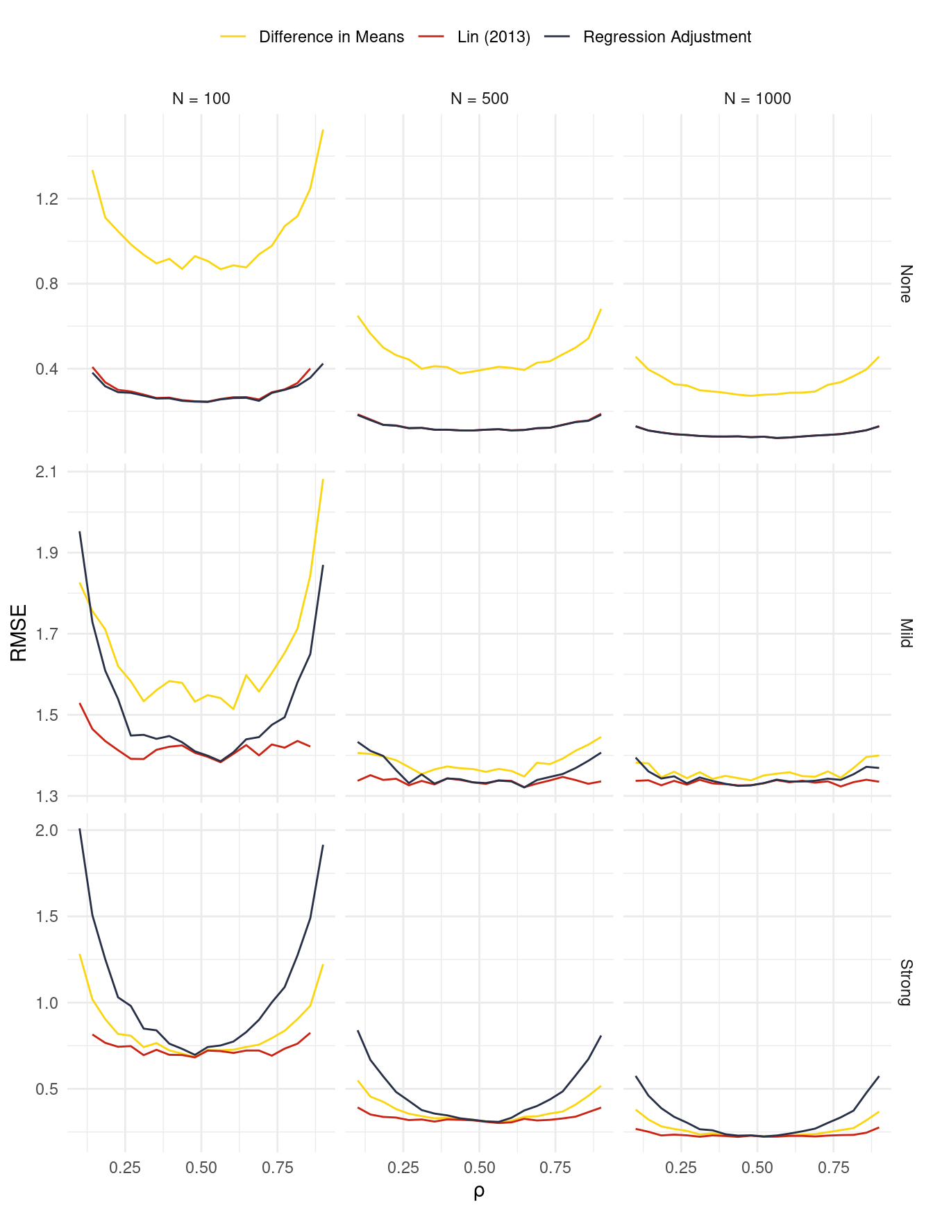
Simulation code

library('MASS')
library('estimatr')
library('data.table')
library('future.apply')
plan(multicore, workers = 5)

simulate = function(
  N = 100,
  rho = 0.1,
  heterogeneity = "Strong") {

  # coefficient heterogeneity
  gamma = list(
    None = list(
      Y0 = c(2, 2, -2, -.05, -.02, .3),
      Y1 = c(3, 2, -2, -.05, -.02, .3)),
    Mild = list(
      Y0 = c(2, 2, -2, -.05, -.02, .3),
      Y1 = c(3, 1, -1, -.05, -.03, -.6)),
    Strong = list(
      Y0 = c(0, 1, -1, -.05, .02, .6),
      Y1 = c(1, -1, 1.5, .03, -.02, -.6)))

  g0 = gamma[[heterogeneity]]$Y0
  g1 = gamma[[heterogeneity]]$Y1

  # correlated covariates
  dat = data.table(mvrnorm(
    n = N, 
    mu = c(1, 2), 
    Sigma = matrix(c(2, .5, .5, 3), ncol = 2)))
  colnames(dat) = c("X1", "X2")

  # treatment 
  dat[, W := rbinom(N, 1, prob = rho)]

  # outcome
  Z = model.matrix(~X1 + X2 + I(X1^2) + I(X2^2) + X1:X2, dat)
  dat[, Y0 := Z %*% g0 + rnorm(N)][
      , Y1 := Z %*% g1 + rnorm(N)][
      , Y  := W * Y1 + (1 - W) * Y0]

  return(dat)
}


fit = function(dat) {
  out = data.table(
    sdim = dat[, mean(Y[W == 1]) - mean(Y[W == 0])],
    ra = coef(lm(Y ~ W + X1 + X2, dat))["W"],
    lin = coef(lm_lin(Y ~ W, ~X1 + X2, dat))["W"]
  )
  return(out)
}


montecarlo = function(
  nsims = 1000,
  N = 100,
  rho = 0.1,
  heterogeneity = "Strong") {

  results = list()

  for (i in 1:nsims) {
    dat = simulate(
      N = N,
      rho = rho, 
      heterogeneity = heterogeneity)

    out = fit(dat)

    out$idx = i
    out$N = N
    out$rho = rho
    out$heterogeneity = heterogeneity

    results[[i]] = out
  }

  results = rbindlist(results)

  return(results)
}

params = CJ(
  N = c(100, 500, 1000),
  rho = seq(.1, .9, length.out = 20),
  heterogeneity = c("Strong", "Mild", "None"))

results = future_Map(
  montecarlo,
  nsims = 1000,
  N = params$N,
  rho = params$rho,
  heterogeneity = params$heterogeneity,
  future.seed = TRUE)

results = rbindlist(results)

results = melt(results,
  id.vars = c("idx", "N", "rho", "heterogeneity"),
  variable.name = "model")

results = results[!value %in% c(-Inf, Inf), .(
  rmse = sqrt(mean((value - 1)^2)),
  bias = mean(value - 1),
  sd = sd(value)),
  by = .(model, N, rho, heterogeneity)]

results[
  , rmse_relative := rmse / min(rmse),
  by = .(N, rho, heterogeneity)]

References

Freedman, David A. 2008a. “On Regression Adjustments in Experiments with Several Treatments.” The Annals of Applied Statistics, 176–96.
———. 2008b. “On Regression Adjustments to Experimental Data.” Advances in Applied Mathematics 40 (2): 180–93.
Lin, Winston. 2013. “Agnostic Notes on Regression Adjustments to Experimental Data: Reexamining Freedman’s Critique.” Annals of Applied Statistics 7 (1): 295–318. https://doi.org/10.1214/12-AOAS583.
Negi, Akanksha, and Jeffrey M. Wooldridge. 2020. “Revisiting Regression Adjustment in Experiments with Heterogeneous Treatment Effects.” Econometric Reviews 0 (0): 1–31. https://doi.org/10.1080/07474938.2020.1824732.