library(brms)
library(ggplot2)
library(marginaleffects)
library(modelsummary)
theme_set(theme_minimal())

titanic <- read.csv("https://vincentarelbundock.github.io/Rdatasets/csv/Stat2Data/Titanic.csv")
titanic <- subset(titanic, PClass != "*")

f <- Survived ~ SexCode + Age + PClass

mod_prior <- brm(f,
    data = titanic,
    prior = c(prior(normal(0, .2), class = b)),
    cores = 4,
    sample_prior = "only")

mod_posterior <- brm(f,
    data = titanic,
    cores = 4,
prior = c(prior(normal(0, .2), class = b)))Bayesians often advocate for the use of prior predictive checks (Gelman et al. 2020). The idea is to simulate from the model, without using the data, in order to refine the model before fitting. For example, we could draw parameter values from the priors, and use the model to simulate values of the outcome. Then, could inspect those to determine if the simulated outcomes (and thus the priors) make sense substantively. Prior predictive checks allow us to iterate on the model without looking at the data multiple times.
One major challenge lies in interpretation: When the parameters of a model are hard to interpret, the analyst will often need to transform before they can assess if the generated quantities make sense, and if the priors are an appropriate representation of available information.
In this post I show how to use the marginaleffects and brms packages for R to facilitate this process. The benefit of the approach described below is that it allows us to conduct prior predictive checks on the actual quantities of interest. For example, if the ultimate quantity that we want to estimate is a contrast or an Average Treatment Effect, then we can use marginaleffects to simulate the specific quantity of interest using just the priors and the model.
In this example, we create two model objects with brms. In one of them, we set sample_prior="only" to indicate that we do not want to use the dataset at all, and that we only want to use the priors and model for simulation:
Now, we use the avg_comparisons() function from the marginaleffects package to compute contrasts of interest:
cmp <- list(
    "Prior" = avg_comparisons(mod_prior),
    "Posterior" = avg_comparisons(mod_posterior))
Finally, we compare the results with and without the data in tables and plots:
modelsummary(
    cmp,
    output = "markdown",
    statistic = "conf.int",
    fmt = fmt_significant(2),
    gof_map = NA,
shape = term : contrast ~ model)| Prior | Posterior | |
|---|---|---|
| Age +1 | 0.0024 | -0.0058 |
| [-0.3810, 0.4155] | [-0.0079, -0.0037] | |
| PClass 2nd - 1st | 0.0031 | -0.19 |
| [-0.3940, 0.3917] | [-0.27, -0.12] | |
| PClass 3rd - 1st | 0.0021 | -0.38 |
| [-0.3714, 0.3794] | [-0.45, -0.31] | |
| SexCode 1 - 0 | 0.00077 | 0.49 |
| [-0.39562, 0.39821] | [0.44, 0.55] |
draws <- lapply(names(cmp), \(x) transform(get_draws(cmp[[x]]), Label = x))
draws <- do.call("rbind", draws)

ggplot(draws, aes(x = draw, color = Label)) +
    xlim(c(-1, 1)) +
    geom_density() +
    facet_wrap(~term + contrast, scales = "free")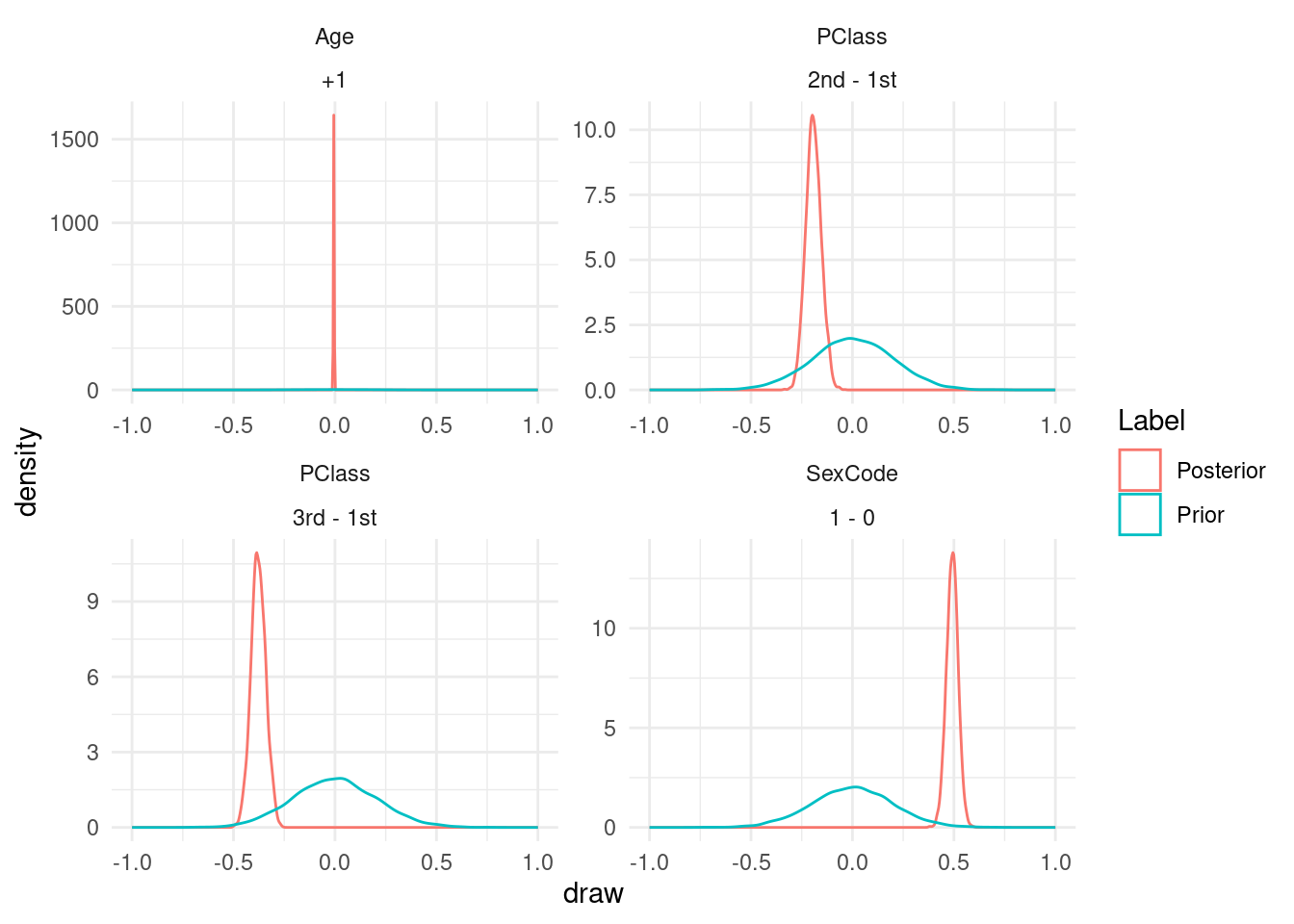
This kind of approach is particularly useful with more complicated models, such as this one with categorical outcomes. In such models, it would be hard to know if a normal prior is appropriate for the different parameters:
modcat_posterior <- brm(
    PClass ~ SexCode + Age,
    prior = c(
        prior(normal(0, 3), class = b, dpar = "mu2nd"),
        prior(normal(0, 3), class = b, dpar = "mu3rd")),
    family = categorical(link = logit),
    cores = 4,
    data = titanic)

modcat_prior <- brm(
    PClass ~ SexCode + Age,
    prior = c(
        prior(normal(0, 3), class = b, dpar = "mu2nd"),
        prior(normal(0, 3), class = b, dpar = "mu3rd")),
    family = categorical(link = logit),
    sample_prior = "only",
    cores = 4,
    data = titanic)
pd <- get_draws(comparisons(modcat_prior))
comparisons(modcat_prior) |> summary() rowid term group contrast
Min. : 1.0 Length:4536 Length:4536 Length:4536
1st Qu.:189.8 Class :character Class :character Class :character
Median :378.5 Mode :character Mode :character Mode :character
Mean :378.5
3rd Qu.:567.2
Max. :756.0
estimate conf.low conf.high rownames
Min. :-5.676e-03 Min. :-8.209e-01 Min. :1.169e-05 Min. : 1.0
1st Qu.: 0.000e+00 1st Qu.:-3.574e-01 1st Qu.:1.711e-02 1st Qu.: 248.8
Median : 0.000e+00 Median :-9.820e-02 Median :9.987e-02 Median : 523.0
Mean :-3.748e-06 Mean :-2.047e-01 Mean :2.049e-01 Mean : 520.5
3rd Qu.: 0.000e+00 3rd Qu.:-1.746e-02 3rd Qu.:3.414e-01 3rd Qu.: 746.2
Max. : 4.333e-03 Max. :-1.609e-05 Max. :8.423e-01 Max. :1313.0
Name PClass Age Sex
Length:4536 Length:4536 Min. : 0.17 Length:4536
Class :character Class :character 1st Qu.:21.00 Class :character
Mode :character Mode :character Median :28.00 Mode :character
Mean :30.40
3rd Qu.:39.00
Max. :71.00
Survived SexCode predicted_lo predicted_hi
Min. :0.000 Min. :0.000 Min. :0.000e+00 Min. :0.000e+00
1st Qu.:0.000 1st Qu.:0.000 1st Qu.:4.000e-09 1st Qu.:4.000e-09
Median :0.000 Median :0.000 Median :1.408e-05 Median :1.503e-05
Mean :0.414 Mean :0.381 Mean :1.572e-02 Mean :1.546e-02
3rd Qu.:1.000 3rd Qu.:1.000 3rd Qu.:2.794e-03 3rd Qu.:2.853e-03
Max. :1.000 Max. :1.000 Max. :1.804e-01 Max. :1.804e-01
predicted tmp_idx
Min. : NA Min. : 1.0
1st Qu.: NA 1st Qu.:189.8
Median : NA Median :378.5
Mean :NaN Mean :378.5
3rd Qu.: NA 3rd Qu.:567.2
Max. : NA Max. :756.0
NA's :4536 comparisons(modcat_posterior) |> summary() rowid term group contrast
Min. : 1.0 Length:4536 Length:4536 Length:4536
1st Qu.:189.8 Class :character Class :character Class :character
Median :378.5 Mode :character Mode :character Mode :character
Mean :378.5
3rd Qu.:567.2
Max. :756.0
estimate conf.low conf.high rownames
Min. :-0.1413142 Min. :-0.216622 Min. :-0.065444 Min. : 1.0
1st Qu.:-0.0122733 1st Qu.:-0.039035 1st Qu.:-0.008223 1st Qu.: 248.8
Median : 0.0005478 Median :-0.008381 Median : 0.005259 Median : 523.0
Mean :-0.0001095 Mean :-0.034000 Mean : 0.035321 Mean : 520.5
3rd Qu.: 0.0263220 3rd Qu.: 0.010666 3rd Qu.: 0.092674 3rd Qu.: 746.2
Max. : 0.1392075 Max. : 0.054036 Max. : 0.226326 Max. :1313.0
Name PClass Age Sex
Length:4536 Length:4536 Min. : 0.17 Length:4536
Class :character Class :character 1st Qu.:21.00 Class :character
Mode :character Mode :character Median :28.00 Mode :character
Mean :30.40
3rd Qu.:39.00
Max. :71.00
Survived SexCode predicted_lo predicted_hi
Min. :0.000 Min. :0.000 Min. :0.02479 Min. :0.02696
1st Qu.:0.000 1st Qu.:0.000 1st Qu.:0.21608 1st Qu.:0.22366
Median :0.000 Median :0.000 Median :0.29571 Median :0.31335
Mean :0.414 Mean :0.381 Mean :0.33301 Mean :0.33288
3rd Qu.:1.000 3rd Qu.:1.000 3rd Qu.:0.45999 3rd Qu.:0.42046
Max. :1.000 Max. :1.000 Max. :0.89623 Max. :0.90880
predicted tmp_idx
Min. : NA Min. : 1.0
1st Qu.: NA 1st Qu.:189.8
Median : NA Median :378.5
Mean :NaN Mean :378.5
3rd Qu.: NA 3rd Qu.:567.2
Max. : NA Max. :756.0
NA's :4536 References
Gelman, Andrew, Aki Vehtari, Daniel Simpson, Charles C. Margossian, Bob Carpenter, Yuling Yao, Lauren Kennedy, Jonah Gabry, Paul-Christian Bürkner, and Martin Modrák. 2020. “Bayesian Workflow.” https://arxiv.org/abs/2011.01808.