library(ggplot2)
library(insight)
library(quantreg)
library(patchwork)
library(marginaleffects)Warning: This notebook is not authoritative. I am very new to conformal inference, and this is just my attempt to work things out (in public). Let me know if you spot mistakes.
Conformal prediction is
“a user-friendly paradigm for creating statistically rigorous uncertainty sets/intervals for the predictions of such models. Critically, the sets are valid in a distribution-free sense: they possess explicit, non-asymptotic guarantees even without distributional assumptions or model assumptions (Angelopoulos & Bates, 2022)”
This is kind of amazing. As I show below, we can get prediction sets with good coverage even if our model is misspecified! The main caveats appear to be that we need iid (or exchangeable) data, and that the tightness of the prediction set will be determined by the quality of a “conformity score” function and of the initial estimator.
This notebook shows several worked examples of split conformal inference, using different score functions to build predictions sets about a mean, linear regression, logitistic regression, and quantile regression. We will only focus on computation; for theory and intuition, interested readers can turn to the reference list at the end of this notebook.
Mean
Take two samples \(X\) and \(Z\) of length \(n\), produced by the same data generating process. Our goal is to use the information in \(X\) to build a prediction set which will cover a proportion of \(Z\) equal to \(1-\alpha\), for a user-specified error rate \(\alpha\). To achieve this, we proceed as follows:
- Split \(X\) into two roughly equal-sized training and calibration datasets.
- Using the training set, estimate the mean \(\bar{X}_t\).
- Using the calibration set, estimate the “conformity score” of each observation.
- The conformity score measures the extent to which observations in the calibration set “conform” to the model estimated in the training set.
- More “informative” conformity score functions tend to produce tighter prediction sets.
- In this example, we use the squared deviation from the training mean as the score.
- Sort observations in the calibration set by their score and let \(d\) equal the absolute residual of the \(k^{th}\) element of the calibration set, with \(k=(n/2 + 1)(1 − \alpha)\).
- Prediction set: \([\bar{X}_t - d, \bar{X}_t + d]\)
Code
conformal <- function(X, alpha = 0.05) {
    # split the original data randomly in two roughly equal parts
    idx <- sample(c(rep(FALSE, floor(length(X) / 2)), rep(TRUE, ceiling(length(X) / 2))))
    X_train <- X[idx]
    X_calib <- X[!idx]
    # fit a new model in the training set
    X_bar <- mean(X_train)
    # conformity score in calibration set: squared residual
    # d: absolute residual
    conf <- data.frame(
        d = abs(X_calib - X_bar),
        score = (X_calib - X_bar)^2)
    # nth conformity score and d
    conf <- conf[order(conf$score), ]
    idx <- ceiling(((length(X) / 2) + 1) * (1 - alpha))
    d <- conf$d[idx]
    # bounds
    out <- c(X_bar - d, X_bar + d)
    return(out)
}
Prediction sets
Now we can call the conform() function to compute prediction sets for arbitrary \(X\) vectors. Of course, the results will differ based on the mean and standard deviation of our datasets:
conformal(rnorm(100, mean = 0, sd = 1))[1] -2.550009 2.416109conformal(rnorm(100, mean = 10, sd = 1))[1] 7.715495 11.931520conformal(rnorm(100, mean = 0, sd = 10))[1] -23.54783 18.95530Coverage
We can check the coverage of those bounds by running some simulations. The next function generates two separate samples: \(X\) and \(Z\). Then, it builds prediction sets using \(X\), and checks if the values in \(Z\) fall within the bounds of that set. Finally, we report the mean covedrage across 1000 simulations. We repeat the experiment a few times with different parameters of the data generation function, and with :
simulate <- function(mean = 0, sd = 1, N = 1000, alpha = .05) {
    X <- rnorm(N, mean = mean, sd = sd)
    Z <- rnorm(N, mean = mean, sd = sd)
    bounds <- conformal(X, alpha = alpha)
    out <- Z > bounds[1] & Z < bounds[2]
    return(out)
}

# Different DGP parameters
mean(replicate(1000, simulate()))
[1] 0.950151mean(replicate(1000, simulate(mean = 10, sd = 1)))[1] 0.950297mean(replicate(1000, simulate(mean = 0, sd = 10)))[1] 0.95069# Different error rate
mean(replicate(1000, simulate(alpha = .1)))[1] 0.900294In all cases, the average coverage hovers around \(1-\alpha\).
Linear regression
To build prediction sets for a linear regression model, we proceed in the same was as above. Fit a model in the training set, and use quantiles of the residuals in the calibration set to construct bounds.
Code
conformal <- function(model, newdata, alpha = 0.05) {
    # compute bounds using the original data and model
    dat <- insight::get_data(model)
    response <- insight::find_response(model)
    # split the original data randomly in two roughly equal parts
    idx <- sample(c(rep(FALSE, floor(nrow(dat) / 2)), rep(TRUE, ceiling(nrow(dat) / 2))))
    dat_train <- dat[idx, ]
    dat_calib <- dat[!idx, ]
    # fit a new model in training split
    mod <- update(model, data = dat_train)
    # conformity score in calibration split: squared residuals
    # d: absolute residuals
    conf <- predictions(
        mod,
        vcov = FALSE,
        newdata = dat_calib)
    conf$score <- residuals(mod)^2
    conf$d <- abs(residuals(mod))
    # nth conformity score and d
    conf <- conf[order(conf$score), ]
    idx <- ceiling(((nrow(dat) / 2) + 1) * (1 - alpha))
    d <- conf$d[idx]
    # add bounds around predictions made on new data
    out <- predictions(
        mod,
        vcov = FALSE,
        newdata = newdata)
    out$conf.low <- out$estimate - d
    out$conf.high <- out$estimate + d
    return(out)
}
Illustration
Consider a correctly-specified linear regression model with polynomial terms, fit on simulated data:
set.seed(1024)

# simulate two datasets
N <- 100

X <- rnorm(N)
past <- data.frame(
    X = X,
    Y = X + X^2 + X^3 + rnorm(N))

X <- rnorm(N)
future <- data.frame(
    X = X,
    Y = X + X^2 + X^3 + rnorm(N))

# fit model
model <- lm(Y ~ X + I(X^2) + I(X^3), data = past)
We first use the predictions() function from the marginaleffects package to build the usual confidence interval around fitted values (displayed in orange below). This interval captures uncertainty around the conditional mean function, but not the irreducible noise that is contained in individual observations. As such, this interval will undercover the predictions by a considerable amount. In contrast, the conformal sets provide adequate coverage for predicted values in new datasets.
# predictions on a grid of predictions, using the original model
pred <- predictions(model)

# use conformal inference to build prediction sets
conf <- conformal(model, newdata = future)

# display results
ggplot(pred) +
    geom_ribbon(data = conf, aes(x = X, ymin = conf.low, ymax = conf.high), alpha = .1, fill = "black") +
    geom_ribbon(aes(x = X, ymin = conf.low, ymax = conf.high), fill = "orange") +
    geom_point(aes(X, Y), alpha = .5) +
    geom_line(aes(X, estimate)) +
    xlim(-2, 2)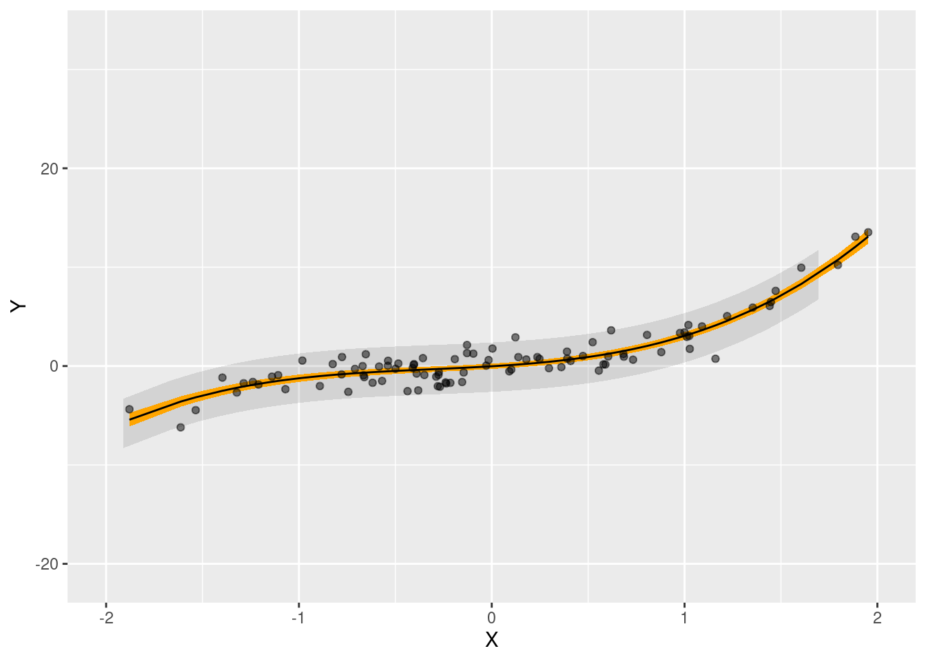
Coverage and Misspecification
One great benefit of conformal inference is that it can yield prediction sets with valid coverage under very minimal assumptions, and even when the model is misspecified. The function below simulates data based on a linear model with polynomial terms. Then, it constructs bounds using two different models: a correctly specified model and a misspecified model without polynomial terms.
simulate <- function(misspecified = FALSE, N = 1000) {
    # past: data used to compute bounds
    X <- rnorm(N)
    past <- data.frame(
        X = X,
        Y = X + X^2 + X^3 + rnorm(N))
    # future: data we want to predict on
    X <- rnorm(N)
    future <- data.frame(
        X = X,
        Y = X + X^2 + X^3 + rnorm(N))
    # misspecified model excludes polynomial terms
    if (isTRUE(misspecified)) {
        model <- lm(Y ~ X + I(X^2) + I(X^3), data = past)
    } else {
        model <- lm(Y ~ X, data = past)
    }
    pred <- conformal(
        model = model,
        newdata = future,
        alpha = .05)
    coverage <- pred$Y > pred$conf.low & pred$Y < pred$conf.high
    return(coverage)
}

# correct model
coverage <- replicate(1000, simulate())
mean(coverage)
[1] 0.948552# misspecified model
coverage <- replicate(1000, simulate(misspecified = TRUE))
mean(coverage)[1] 0.9482The coverage rate is about correct, even when the model is misspecified.
Logistic regression
We can build prediction intervals for GLM models as well. For a logistic regression model, we modify the procedure above in 3 ways:
- Use the absolute deviance residuals for conformity scores.
- Use the \(k^{th}\) quantile of the partial residuals as \(d\) value to build the bounds.
- Make predictions on the link scale and backtransform them to make sure that the bounds stay in the \([0, 1]\) interval.
Warning: I am not 100% confident in the choice of partial residuals for \(d\) (mostly because I’m too lazy to read the residuals.glm documentation). If you can confirm or recommend something else, please let me know.
Code
conformal <- function(model, newdata, alpha = 0.05) {
    dat <- insight::get_data(model)
    # split the original data randomly in two roughly equal parts
    idx <- sample(c(rep(FALSE, floor(nrow(dat) / 2)), rep(TRUE, ceiling(nrow(dat) / 2))))
    dat_train <- dat[idx, ]
    dat_calib <- dat[!idx, ]
    # fit a new model on split 1
    mod <- update(model, data = dat_train)
    # conformity score in split 2: absolute residuals
    conf <- predictions(
        mod,
        vcov = FALSE,
        newdata = dat_calib)
    conf$score <- abs(residuals(mod, type = "deviance"))
    conf$d <- abs(residuals(mod, type = "partial"))
    # nth conformity score and d
    conf <- conf[order(conf$score), ]
    idx <- ceiling(((nrow(dat) / 2) + 1) * (1 - alpha))
    d <- conf$d[idx]
    # bounds around link scale predictions on `newdata`
    out <- predictions(
        mod,
        type = "link",
        vcov = FALSE,
        newdata = newdata)
    out$conf.low <- out$estimate - d
    out$conf.high <- out$estimate + d
    # backtransform
    link_inv <- insight::link_inverse(model)
    out$conf.low <- link_inv(out$conf.low)
    out$conf.high <- link_inv(out$conf.high)
    return(out)
}
Illustration
We now simulate data for a simple logistic regression model, and build a standard confidence interval around fitted values, as well as prediction intervals using split conformal inference.
N <- 1000
X <- rnorm(N)
Z <- rnorm(N)
Y <- rbinom(N, 1, plogis(5 * X))
dat <- data.frame(Y, X)
model <- glm(Y ~ X, data = dat, family = binomial)
newdata <- data.frame(Y, X)

# conformal inference
conf <- conformal(model, newdata = newdata)

# confidence intervals around predicted values
pred <- predictions(model, newdata = datagrid(X = seq(-3, 3, length.out = 200)))

p1 <- ggplot(conf, aes(x = X, y = Y, ymin = conf.low, ymax = conf.high)) +
    geom_ribbon(aes(x = X, ymin = conf.low, ymax = conf.high), alpha = .2) +
    geom_point(alpha = .1) +
    ylab("Conformal interval")

p2 <- ggplot(pred, aes(x = X, y = estimate, ymin = conf.low, ymax = conf.high)) +
    geom_ribbon(alpha = .2) +
    geom_line() +
    ylab("Confidence interval")

p1 / p2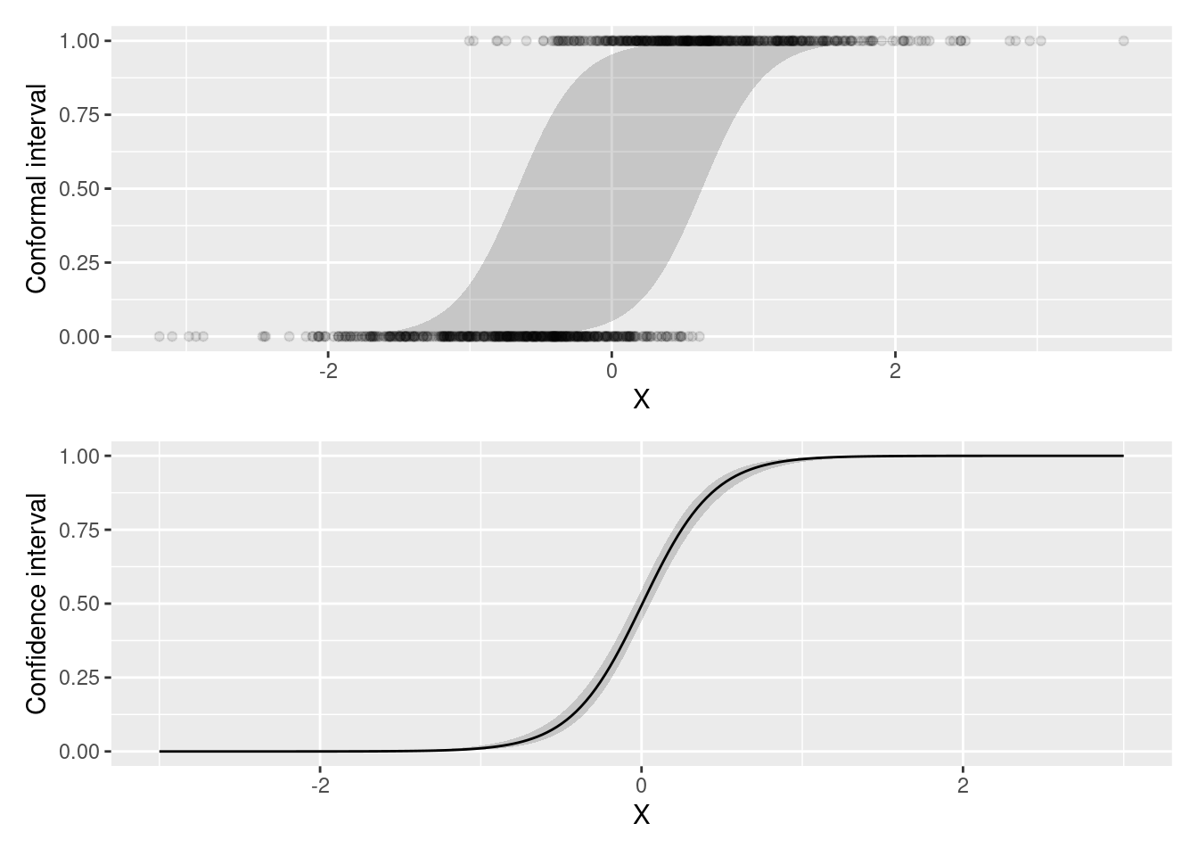
Quantile regression
The code below is an attempt to apply the procedure and check the bounds suggested in:
- Romano, Yaniv, Evan Patterson, and Emmanuel Candes. “Conformalized Quantile Regression.” In Advances in Neural Information Processing Systems, Vol. 32. Curran Associates, Inc., 2019. https://proceedings.neurips.cc/paper/2019/hash/5103c3584b063c431bd1268e9b5e76fb-Abstract.html.
In a very simple simulation the coverage seems fine, but I make no guarantees that the code works as intended. Please let me know if you spot mistakes.
set.seed(1024)

conformal <- function(model, newdata, alpha = 0.05) {
    # get the original data and the name of the response variable
    dat <- insight::get_data(model)
    response <- insight::find_response(model)
    # split the original data randomly in two roughly equal parts
    idx <- sample(c(rep(FALSE, floor(nrow(dat) / 2)), rep(TRUE, ceiling(nrow(dat) / 2))))
    dat_train <- dat[idx, ]
    dat_calib <- dat[!idx, ]
    # fit two conditional quantile functions in the training split
    mod.low <- update(model, tau = alpha / 2, data = dat_train)
    mod.high <- update(model, tau = (1 - alpha / 2), data = dat_train)
    # conformity score in calibration split: absolute residuals
    # d and score are the same
    pred.low <- predictions(mod.low, vcov = FALSE, newdata = dat_calib)
    pred.high <- predictions(mod.high, vcov = FALSE, newdata = dat_calib)
    conf <- predictions(model, vcov = FALSE, newdata = dat_calib)
    conf$predicted.low <- pred.low$estimate
    conf$predicted.high <- pred.high$estimate
    conf$d <- conf$score <- pmax(
        conf[["predicted.low"]] - conf[[response]],
        conf[[response]] - conf[["predicted.high"]])
    # nth conformity score and d
    conf <- conf[order(conf$score), ]
    idx <- ceiling(((nrow(dat) / 2) + 1) * (1 - alpha))
    d <- conf$d[idx]
    # bounds around predictions on `newdata`
    conf$conf.low <- conf$predicted.low - d
    conf$conf.high <- conf$predicted.high + d
    return(conf)
}

simulate <- function(N = 1000) {
    # data used to compute bounds
    X <- rnorm(N)
    dat_past <- data.frame(
        X = X,
        Y = X + X^2 + X^3 + rnorm(N))
    # data we want to predict on
    X <- rnorm(N)
    dat_future <- data.frame(
        X = X,
        Y = X + X^2 + X^3 + rnorm(N))
    model <- rq(Y ~ X + I(X^2) + I(X^3), data = dat_past)
    pred <- conformal(
        model = model,
        newdata = dat_future,
        alpha = .05)
    coverage <- pred$Y > pred$conf.low & pred$Y < pred$conf.high
    return(coverage)
}

coverage <- replicate(1000, simulate())
mean(coverage)
[1] 0.95N <- 1000
X <- seq(-3, 3, length.out = N)
past <- data.frame(
X = X,
Y = X + X^2 + X^3 + rnorm(N))
X <- seq(-3, 3, length.out = N)
future <- data.frame(
X = X,
Y = X + X^2 + X^3 + rnorm(N))
model <- rq(Y ~ X + I(X^2) + I(X^3), data = past)
conf <- conformal(model, newdata = future)
ggplot(conf) +
geom_ribbon(aes(x = X, ymin = conf.low, ymax = conf.high), alpha = .3) +
geom_ribbon(aes(x = X, ymin = predicted.low, ymax = predicted.high), fill = "orange") +
geom_point(aes(x = X, y = Y), alpha = .3) +
ggtitle("Grey: Conformal prediction set\nOrange: Quantile regression interval")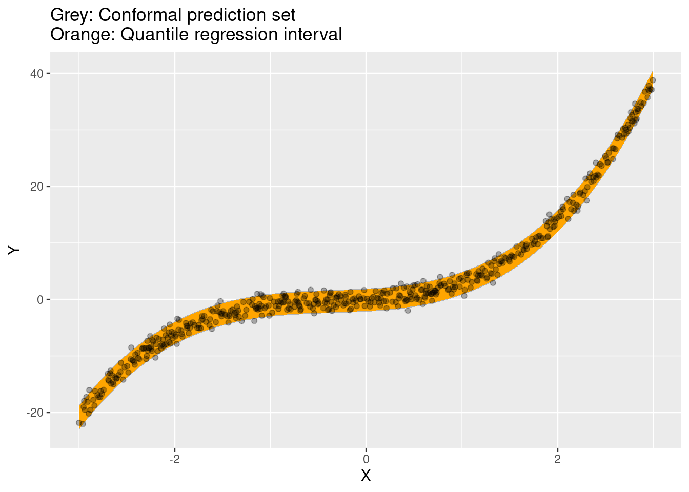
References
- Samii, Cyrus. “Conformal Inference Tutorial.” https://cdsamii.github.io/cds-demos/conformal/conformal-tutorial.html
- Angelopoulos, Anastasios N., and Stephen Bates. “A Gentle Introduction to Conformal Prediction and Distribution-Free Uncertainty Quantification.” arXiv, September 3, 2022. https://doi.org/10.48550/arXiv.2107.07511.
- Lei, Jing, Max G’Sell, Alessandro Rinaldo, Ryan J. Tibshirani, and Larry Wasserman. “Distribution-Free Predictive Inference for Regression.” Journal of the American Statistical Association 113, no. 523 (July 3, 2018): 1094–1111. https://doi.org/10.1080/01621459.2017.1307116.
- Romano, Yaniv, Evan Patterson, and Emmanuel Candes. “Conformalized Quantile Regression.” In Advances in Neural Information Processing Systems, Vol. 32. Curran Associates, Inc., 2019. https://proceedings.neurips.cc/paper/2019/hash/5103c3584b063c431bd1268e9b5e76fb-Abstract.html.
- Shafer, Glenn, and Vladimir Vovk. “A Tutorial on Conformal Prediction.” arXiv, June 21, 2007. https://doi.org/10.48550/arXiv.0706.3188.